1 Introduction to R
1.1 Why R?
In this chapter we will discuss the basics of R programming. R is a free software, used by millions in the field of statistics, data science, economics and many others.
The R programming language is an important tool for data related tasks, but it is much more. Just like other programming languages, R has many additional packages, which can extend its basic functionality. R has a great (probably the best) graphical tools to create your charts, and with shiny, you can easily build your minimalist web applications. We will learn about data manipulation, analysis and how to create awesome reports, like dashboards.
1.2 Setup
You can download R and RStudio from the official site of RStudio. Please install the appropriate version based on your OS, and do not forget that you also have to install R as well.


Run R’s installer file after the downloading process is finished. Next, we will also need the RStudio.

If the installation process of R and RStudio is finished, then we can open RStudio and start to learn the software.
1.3 Our first meet with R
RStudio is dedicated IDEE for R, which means, that it will make our life much simplier. In stead of writing each line of code ourself, RStudio has many built-in functions to help us. We see some panes if we open RStudio:
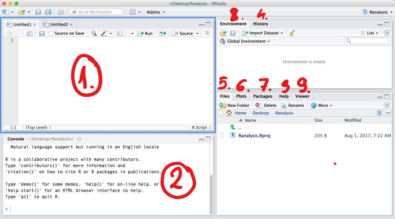
Figure 1.1: Panes in RStudio
-
Source
- We will write here our codes, which we would like to save.
The basic extension of our codes are
.R, but this is not the only possibility (we will cover this later). Once you save your code for later use, you can open your script also with a simple text editor (like Notepad), since this is only plain text. If you hitenteryour code wont be executed, you will just simply start a new line. If you want to run your code hitctrl + enterto execute a single line, andctrl+shift+enterto execute your full script.
- We will write here our codes, which we would like to save.
The basic extension of our codes are
-
Console
- Here you find the executed codes, and the response to that. For example, if you type
2 + 2and hitenter, R will execute the expression, and response that it is 4.
- Here you find the executed codes, and the response to that. For example, if you type
2 + 2
#> [1] 4-
Help
- You can use this pane if you are not familier with a function. For example, you want to know what input you can specify while using
mean, you can type?meanon the console, or use the search field on this pane. The description of the function will be presented on this pane. (This pane is super useful on the exam)
- You can use this pane if you are not familier with a function. For example, you want to know what input you can specify while using
History
-
Files
- You can see the list of your files which are in the current working directory. Working directory is the folder, from where R want currently read the files. If you want to import a dataset, just click on a file on this pane.
- I highly recommend you to set a project folder for the class and any later job. This means that, R creates a folder and puts an
.Rprojfile into it. You can always click on this.Rprojfile to return your unfinished work. You can customise if R should put the variables into your environtent as you left them last time, you have a history about the used codes, and you see all the data you copy + paste into this folder.
Plots
-
Packages
- You can install packages from this pane. If you need a given package, click on install, and start typing its name. After that, you have to activate packages each time you open R again with the
library(eurostat)command. You can also use a function from a package if you just simly typeeurostat::get_eurostat().
- You can install packages from this pane. If you need a given package, click on install, and start typing its name. After that, you have to activate packages each time you open R again with the
-
Environment
- Here you can see the list of the variables you have already created. For example you can type
x = 3on the console. Now and x variable will appear in the environment pane, and you can check its value if you typexon the console. You can also save these variables into an.RDatadata format if you wish.
- Here you can see the list of the variables you have already created. For example you can type
Viewer
1.4 Data types
Lets see first, what kind of datatypes exist in R. Lets assign a variable called x.
x <- 4So, what is the type of x? We can use the class command to answer this.
class(x)
#> [1] "numeric"
Its numeric1. This means that you can use +, -, * operators on it.
Lets see other types.
y <- "blue"
class(y)
#> [1] "character"
Its a character, basically can contain any kind of letter, digits, or white space.
does_it_rain <- TRUE
class(does_it_rain)
#> [1] "logical"
Its a logical value. It can be TRUE or FALSE
1.4.1 vectors
We can create a vector with the c function. (combine)
x <- c(11, 201, 301)
x
#> [1]  11 201 301
We can asses a given element of it by:
x[2]
#> [1] 201
Or we can use functions on it:
sum(x)
#> [1] 513
We can also easily create sequence with the syntax start:stop
1:10
#>  [1]  1  2  3  4  5  6  7  8  9 10
If we combine characters, I mentiont that we can convert this vector to factor type. This is useful if we can enclose an order to the vector or we want to control for the possible values. Lets see a minimal example
my_vector <- c("First", "Second", "Third", "Fourth")
sort(my_vector)
#> [1] "First"  "Fourth" "Second" "Third"
If we want to sort the vector, we see that Fourth comes right after First. It is because character vectors are sorted in alphabetical order. We can solve it with factor
my_vector2 <- factor(my_vector, ordered = TRUE, levels = c("First", "Second", "Third", "Fourth"))
sort(my_vector2)
#> [1] First  Second Third  Fourth
#> Levels: First < Second < Third < Fourth
We can merge these vectors into a data.frame, which is basically like an excel table. Each column is a variable (with a header), and each row is an observation.
avengers_df <- data.frame(name = c("Captain America", "Hulk", "Dr. Strange"),
           color = c("blue", "green", NA))

avengers_df
#>              name color
#> 1 Captain America  blue
#> 2            Hulk green
#> 3     Dr. Strange  <NA>
NA stands for “not available”, so these values are missing. Most of the times we will work with data.frames (similarly like pandas in python), so it is the most important data type we learn.
Storing more complex data, you can use the list. To use data.frame you need vectors with equal length. If this does not hold, or a more frequent case, you want to store a collection of data.frames, then list is a perfect solution! It is not a rare issue, big panel dataset are usually stored in separated files (a different file to each year, like: cis_survey2016.csv, cis_survey2017.csv). In this situations its suggested to store your data in a list.
mylist <- list(avengers_df, my_vector, x)Now mylist stores a data.frame and two vector. You can access the components with a [[ ]]. For example, the first element:
mylist[[1]]
#>              name color
#> 1 Captain America  blue
#> 2            Hulk green
#> 3     Dr. Strange  <NA>
1.5 Data manipulation
1.5.1 Import data into R
We mentioned formely that the easiest way to import your data is to click on it in the files pane. However, this manual step is useful if you have to import and analyse the data once, but probably you want to use your data next time as well. That is way it is a good idea to copy and paste the code for importing the data into your script.
Figure 1.2: Import csv data into R
In fact, if the data is in your working directory, you can refer to it with “relative referencing”. This means that you have to type only the name of the file, not the full path, because R will automatically start to look for the file in the working directory2.
library(readr)
df <- read_delim("da_q.csv", delim = ";", escape_double = FALSE, trim_ws = TRUE)
df <- read_delim(str_c(WD, "/data/da_q.csv"), delim = ";", escape_double = FALSE, trim_ws = TRUE)Now we have imported a tidy dataset. Each column is variable, and each row is an observation. Lets see how to select specific data from that. If you want to analyse only one column of it, you can use $ operator.
pizza <- df$`How many slices of pizza can you it at once?`

pizza
#>  [1] "8"
#>  [2] "12"
#>  [3] "Depends on size. Can be up to 5 slices of the medium pizza"
#>  [4] "2"
#>  [5] "3"
#>  [6] "4"
#>  [7] "4"
#>  [8] "4"
#>  [9] "3"
#> [10] "2"
#> [11] "4"
#> [12] "3"
#> [13] "3"
#> [14] "2"
#> [15] "2"
#> [16] "4 and It depends how much I am hungry"
#> [17] "4"
#> [18] "3"
#> [19] "2"
#> [20] "6"
#> [21] "3"
The output pizza is a character vector currently, because some of the answers contain letters. We have to options here:
- Using
as.numericfunction to force R using the values as numerical data.
as.numeric(pizza)
#> Warning: NAs introduced by coercion
#>  [1]  8 12 NA  2  3  4  4  4  3  2  4  3  3  2  2 NA  4  3  2  6  3
We got a warning message. Where letters appear R cannot convert the values to numbers, so this values became NA (Not Available) values.
- Remove the letters from the answers and convert the vector to the correct datatype.
To manage this, we have to use the syntax called regular expressions. I want to show you 4 expressions now and a function. The function gsub will detect a given letter in a character and replace it with something. Lets see how!
gsub(x = "Awesome 12", pattern = "\\w", replacement = "B") # every non-white space
#> [1] "BBBBBBB BB"
gsub(x = "Awesome 12", pattern = "\\s", replacement = "B") # every white space
#> [1] "AwesomeB12"
gsub(x = "Awesome 12", pattern = "\\d", replacement = "B") # every digit
#> [1] "Awesome BB"
gsub(x = "Awesome 12", pattern = "\\D", replacement = "B") # every non-digit value
#> [1] "BBBBBBBB12"
So we can use the last example to solve our problem.
pizza_only_digits <- gsub(x = pizza, pattern = "\\D", replacement = "")

pizza_only_digits
#>  [1] "8"  "12" "5"  "2"  "3"  "4"  "4"  "4"  "3"  "2"  "4"  "3"  "3"  "2"  "2"
#> [16] "4"  "4"  "3"  "2"  "6"  "3"

as.numeric(pizza_only_digits)
#>  [1]  8 12  5  2  3  4  4  4  3  2  4  3  3  2  2  4  4  3  2  6  3
1.6 Conditional statements
We offen use conditional statement in programming. It has a clean concept: If the condition is TRUE, then evaluate the following task.
If you want to write an if else statement in R, I highly recomment you to use the snippet for that. Snippet means, that when you type if and press shift + tab, then R will automaticly write the framework you have to use:
if (condition) {

}
As a condition you have to use a logical value as input, or a condition. You can use conditions with the following operators: <, >, <=, >=, ==, !=, is.na, %in%, stringr::str_detect().
4 < 5
#> [1] TRUE
5 <= 5
#> [1] TRUE
4 > 5
#> [1] FALSE
5 >=4
#> [1] TRUE
2 == 3 # equal?
#> [1] FALSE
(2 + 2) == 4
#> [1] TRUE
(2 + 2) != 4 # not equal?
#> [1] FALSE
3 != 3
#> [1] FALSE
is.na(4)
#> [1] FALSE
is.na(NA)
#> [1] TRUE
3 %in% c(1, 2, 3)
#> [1] TRUE
stringr::str_detect(string = "this function is awesome!", pattern = "some")
#> [1] TRUE
stringr::str_detect(string = "this function is awesome!", pattern = "none")
#> [1] FALSE
You can also specify the task R has to do, if the statement is false.
1.7 Loops
1.7.1 While
You can also use while loop to specify a task R has to do until a condition is TRUE.
x <- 1

while (x < 15) {
  cat(paste0(x, "^2=")) # cat = print, just into the same line
  cat(x^2)
  cat("\n") # force R to create a new line
  x <- x + 1 # if you miss this step then R will repeat the task infinit times
}
#> 1^2=1
#> 2^2=4
#> 3^2=9
#> 4^2=16
#> 5^2=25
#> 6^2=36
#> 7^2=49
#> 8^2=64
#> 9^2=81
#> 10^2=100
#> 11^2=121
#> 12^2=144
#> 13^2=169
#> 14^2=196
1.7.2 For
With this framewrok you can specify a task, that R has to do x times. For example, print a message 10 times.
for (i in 1:10) {
  print("You R amazing!")
}
#> [1] "You R amazing!"
#> [1] "You R amazing!"
#> [1] "You R amazing!"
#> [1] "You R amazing!"
#> [1] "You R amazing!"
#> [1] "You R amazing!"
#> [1] "You R amazing!"
#> [1] "You R amazing!"
#> [1] "You R amazing!"
#> [1] "You R amazing!"
And you can use i inside the { parenthesis.
for (i in 1:5) {
  print(i)
}
#> [1] 1
#> [1] 2
#> [1] 3
#> [1] 4
#> [1] 5
1.8 Functions
We offen work with functions in R, but you can also write your own. You have to use the function word and specify the input variables.
my_first_function <- function(x) {
  # removed all non-digit characters from x, and take the squared of it.
  as.numeric(gsub(x, pattern = "\\D", replacement = ""))^2
}

my_first_function("Depends on, maybe 5 slices")
#> [1] 25
1.9 Apply family
This family contains 3 functions, which I want to show you (There are more complex ones, those are not covered in this bookdown).
The function apply tells R to use a function on each row or column of a data.frame. So the its frist argument is the data.frame, the third is the function which shoul use and the second is the margin:
- margin = 2: apply the given function on each of the COLUMNS
- margin = 1: apply the given function on each of the ROWS
non_na <- function(x) {
  # how many numeric observation are in the vector
  sum(!is.na(as.numeric(x)))
}
Number of numeric answers by quetions:
apply(df, 2, non_na)
#>                                                                                ID
#>                                                                                21
#>                    What is your zodiac? (https://www.astrology-zodiac-signs.com/)
#>                                                                                 0
#>                                                       Do you prefer dogs or cats?
#>                                                                                 0
#>                             What experiences do have on related to R programming?
#>                                                                                 0
#>                                      How many slices of pizza can you it at once?
#>                                                                                19
#>                                                             Do you wear glasses?2
#>                                                                                 0
#>                                       How many countries have you been to so far?
#>                                                                                21
#>   How many instagram followers do you have? (zero, if you do not have an account)
#>                                                                                20
#>                                        How many brothers and sisters do you have?
#>                                                                                19
#>                              What is your batteries current charge level? (0-100)
#>                                                                                19
#> What is the traditional food in your country? (you can mention more, if you wish)
#>                                                                                 0
Number of numeric answers by participant:
apply(df, 1, non_na)
#>  [1] 6 6 4 5 6 6 6 6 6 6 5 6 6 6 6 4 6 6 6 6 5
Lapply is similar but with list objects.
mylist <- list(
  first_vector = c(1, 2, 3),
  second_vector = letters # built in character vector, contains all the letters
)

mylist
#> $first_vector
#> [1] 1 2 3
#>
#> $second_vector
#>  [1] "a" "b" "c" "d" "e" "f" "g" "h" "i" "j" "k" "l" "m" "n" "o" "p" "q" "r" "s"
#> [20] "t" "u" "v" "w" "x" "y" "z"
We are interested in the number of observation (the length) of each vector:
out <- lapply(mylist, length)

out
#> $first_vector
#> [1] 3
#>
#> $second_vector
#> [1] 26

class(out)
#> [1] "list"
But the output is still a list. sapply is the solution if we want to convert it into vector.
sapply(mylist, length)
#>  first_vector second_vector
#>             3            26