2 Markdown & Tidyverse
2.1 Markdown
Last week we wrote or codes on the Source pane, and if you save the codes and revisit the file with your file explorer, you can see that the extension of the file is .R. You can open the file with any other text editor (like Notepad) and see the codes. In a .R file you can write your codes and comments, and if you hit ctrl + shift + enter then all lines will be evaluated. Most of the times the goal to use .R files is this, we want to reuse the codes frequently (like downloading data from a website).
Another possible extension for your files is the .Rmd, which stands for R MarkDown. In this file format you can combine text, R codes and their output into one single document. from now, We will use RMarkdown during the class. Please visit the following website to find useful examples: https://rmarkdown.rstudio.com/articles_intro.html
2.2 Introduction to the tidyverse
We will work with the tidyverse today. You can simply install it from the CRAN (go to Packages pane and click the install button). But tidyverse is not a simple package. “The tidyverse is a set of packages that work in harmony because they share common data representations […]”
Tidyverse contains the most important packages that you’re likely to use in everyday data analyses:
ggplot2, for data visualisation.
dplyr, for data manipulation.
tidyr, for data tidying.
readr, for data import.
purrr, for functional programming.
tibble, for tibbles, a modern re-imagining of data frames.
stringr, for strings.
forcats, for factors.
After you installed the packages, you can load in the core packages with `library` command. You will receive a warning message, but do not worry, this is fine.
2.3 The %>% operator
This operator is written ctrl + shift + m, it is denoted as %>%, but we pronounce as pipe. To understand its relevance, you should think about it like … then. This opreator forward the value of the previous expression into the next function as the first unspecified input. Lets see an example:
We first generate a numerical vector as trajectories of standard normal distribution.
norm_sample <- rnorm(n = 1000, mean = 0, sd = 1) # standard normalAND THEN we visualize its distribution with a histogram.
hist(norm_sample)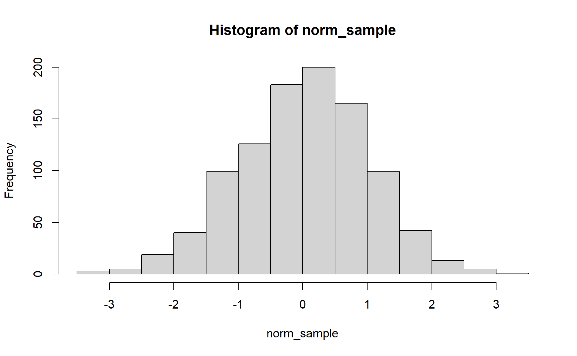
Figure 2.1: Histogram of standard normal distribution
Now we had to assign the norm_sample object to use only for a single graph. If you are working on a project it will be confusing to have tons of one time used objects in your environment (Like DataFrameAfterCleaningStep1, DataFrameAfterCleaningStep2, DataFrameAfterCleaningStep3, etc.).
With the pipe operator we can embed several steps into one single workflow. This way we do not have to assign the norm_sample object. We simple generate the random values AND THEN draw their distribution.
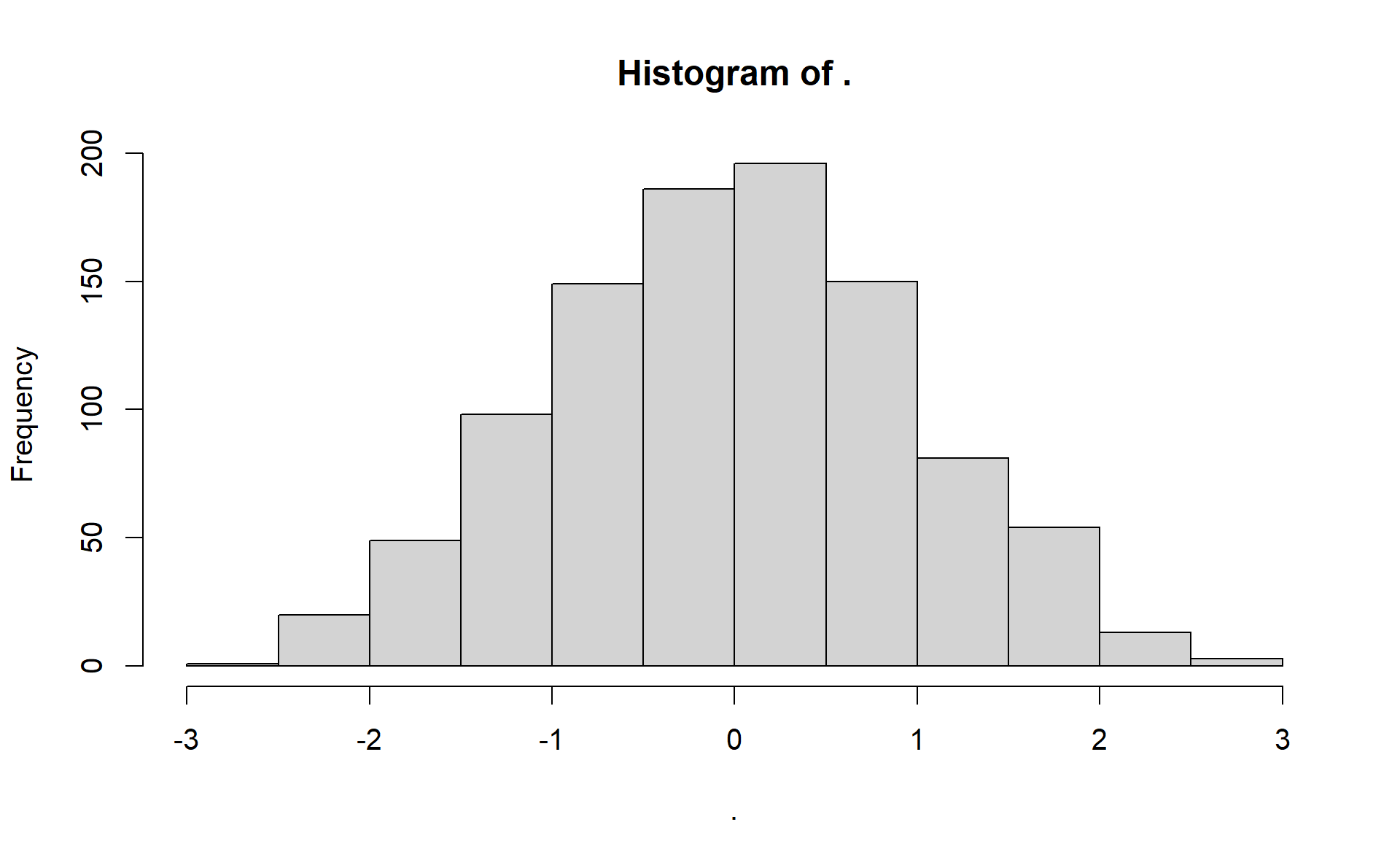
Figure 2.2: Histogram of standard normal distribution using the pipe
You may see that the title of plot has changed (probably the graph also changed a bit, since chances are low that we generate exactly the 1000 random values). This is because pipe and many other tidyverse function works with a lambda like function framework. This means that you can refer to the input value (only if you have only one single input) with ..
Example:
(2 + 2) %>%
  {. * .}
#> [1] 16
The result is 16, since 2 + 2 = 4, and 4 * 4 equals 16.
The pipe may seem unrelevant first, but this is one of the most powerful tool in R if you have complex data manipulating steps. We will cover the core functions of dplyr in this chapter, which appear in the following video (37:30 - 38:30), but when you are familier with them, you will see the motivation behind the pipe.
2.4 Tibble, count, filter, select, arrange
2.4.1 Tibble
Let’s import a dataset from the OECD webpage. Download the data in csv format and paste it into your working directory.
fertility_df <- read_csv("DP_LIVE_22092021161631568.csv")read_csv is importad from the readr package, thus shares its output is adequat to the tidyverse principles. fertility_df is a data.frame, but it is a tibble, which means that it will be printed nicely on the console: only the first 10 rows appears, and only the amount of columns that can be printed without a linebreak (similar to pandas dataframe in python).
fertility_df
#> # A tibble: 3,193 x 8
#>    LOCATION INDICATOR SUBJECT MEASURE   FREQUENCY  TIME Value `Flag Codes`
#>    <chr>    <chr>     <chr>   <chr>     <chr>     <dbl> <dbl> <lgl>
#>  1 AUS      FERTILITY TOT     CHD_WOMAN A          1960  3.45 NA
#>  2 AUS      FERTILITY TOT     CHD_WOMAN A          1961  3.55 NA
#>  3 AUS      FERTILITY TOT     CHD_WOMAN A          1962  3.43 NA
#>  4 AUS      FERTILITY TOT     CHD_WOMAN A          1963  3.34 NA
#>  5 AUS      FERTILITY TOT     CHD_WOMAN A          1964  3.15 NA
#>  6 AUS      FERTILITY TOT     CHD_WOMAN A          1965  2.97 NA
#>  7 AUS      FERTILITY TOT     CHD_WOMAN A          1966  2.89 NA
#>  8 AUS      FERTILITY TOT     CHD_WOMAN A          1967  2.85 NA
#>  9 AUS      FERTILITY TOT     CHD_WOMAN A          1968  2.89 NA
#> 10 AUS      FERTILITY TOT     CHD_WOMAN A          1969  2.89 NA
#> # ... with 3,183 more rows
2.4.2 Count
With the count function you can simple count the number of appearancesof the levels of a given column. Example:
count(fertility_df, LOCATION)
#> # A tibble: 54 x 2
#>    LOCATION     n
#>    <chr>    <int>
#>  1 ARG         60
#>  2 AUS         60
#>  3 AUT         61
#>  4 BEL         60
#>  5 BGR         60
#>  6 BRA         60
#>  7 CAN         60
#>  8 CHE         61
#>  9 CHL         60
#> 10 CHN         60
#> # ... with 44 more rows
Now we can see that we have 60 observation from ARG. If you are interested in for which country we have the most datapoints, you can use the sort = TRUE option.
count(fertility_df, LOCATION, sort = TRUE)
#> # A tibble: 54 x 2
#>    LOCATION     n
#>    <chr>    <int>
#>  1 AUT         61
#>  2 CHE         61
#>  3 CZE         61
#>  4 DNK         61
#>  5 EST         61
#>  6 FIN         61
#>  7 FRA         61
#>  8 LUX         61
#>  9 NOR         61
#> 10 NZL         61
#> # ... with 44 more rows
You can also use the pipe here[^It would not be a good solution to assign a new dataframe to each count table]
fertility_df %>% # %>% = the 1st argument of count function is the fertility_df data.frame
  count(LOCATION)
#> # A tibble: 54 x 2
#>    LOCATION     n
#>    <chr>    <int>
#>  1 ARG         60
#>  2 AUS         60
#>  3 AUT         61
#>  4 BEL         60
#>  5 BGR         60
#>  6 BRA         60
#>  7 CAN         60
#>  8 CHE         61
#>  9 CHL         60
#> 10 CHN         60
#> # ... with 44 more rows
You may specifiy multiple columns, this way the frequency of all value combinaton appears.
fertility_df %>%
  count(LOCATION, TIME, sort = T)
#> # A tibble: 3,193 x 3
#>    LOCATION  TIME     n
#>    <chr>    <dbl> <int>
#>  1 ARG       1960     1
#>  2 ARG       1961     1
#>  3 ARG       1962     1
#>  4 ARG       1963     1
#>  5 ARG       1964     1
#>  6 ARG       1965     1
#>  7 ARG       1966     1
#>  8 ARG       1967     1
#>  9 ARG       1968     1
#> 10 ARG       1969     1
#> # ... with 3,183 more rows
Now we see that we have only one observation for each country at a time, so this data frame was originally tidy (this is usually not the case). Let’s see for example the Q GDP data from the OECD webpage.
gdp_df <- read_csv("DP_LIVE_22092021163414835.csv")Using the count function, we may find that MEASURE, SUBJECT & FREQUENCY columns have multiple levels.
gdp_df %>%
  count(MEASURE, SUBJECT, FREQUENCY)
#> # A tibble: 5 x 4
#>   MEASURE  SUBJECT FREQUENCY     n
#>   <chr>    <chr>   <chr>     <int>
#> 1 IDX      VOLIDX  A          1764
#> 2 IDX      VOLIDX  Q          7127
#> 3 PC_CHGPP TOT     A          2329
#> 4 PC_CHGPP TOT     Q          9472
#> 5 PC_CHGPY TOT     Q          9385
Let’s say we are interested only in the observations where the SUBJECT is equal to TOT (total), MEASURE is equal to PC_CHGPY (percentage change to previous value) and the FREQUENCY is not equal to A (only quarterly observations). You can select rows by using the filter function. Its 1st argument is the dataframe you want to modify, and the other arguments are conditional statements. If all the statements are TRUE, then the row will be selected.
filter(gdp_df, SUBJECT == "TOT", MEASURE == "PC_CHGPY", FREQUENCY != "A")
#> # A tibble: 9,385 x 8
#>    LOCATION INDICATOR SUBJECT MEASURE  FREQUENCY TIME     Value `Flag Codes`
#>    <chr>    <chr>     <chr>   <chr>    <chr>     <chr>    <dbl> <chr>
#>  1 DEU      QGDP      TOT     PC_CHGPY Q         1961-Q1  7.45  E
#>  2 DEU      QGDP      TOT     PC_CHGPY Q         1961-Q2  5.00  E
#>  3 DEU      QGDP      TOT     PC_CHGPY Q         1961-Q3  3.58  E
#>  4 DEU      QGDP      TOT     PC_CHGPY Q         1961-Q4  3.00  E
#>  5 DEU      QGDP      TOT     PC_CHGPY Q         1962-Q1  3.47  E
#>  6 DEU      QGDP      TOT     PC_CHGPY Q         1962-Q2  5.11  E
#>  7 DEU      QGDP      TOT     PC_CHGPY Q         1962-Q3  5.47  E
#>  8 DEU      QGDP      TOT     PC_CHGPY Q         1962-Q4  4.76  E
#>  9 DEU      QGDP      TOT     PC_CHGPY Q         1963-Q1 -0.372 E
#> 10 DEU      QGDP      TOT     PC_CHGPY Q         1963-Q2  3.02  E
#> # ... with 9,375 more rows
Just like the count, we use this function with %>% operator, and use & instead of ,, but if you wish to use “OR”, then you can use | between two statement.
gdp_df %>%
  filter(SUBJECT == "TOT" & MEASURE == "PC_CHGPY" & FREQUENCY != "A")
#> # A tibble: 9,385 x 8
#>    LOCATION INDICATOR SUBJECT MEASURE  FREQUENCY TIME     Value `Flag Codes`
#>    <chr>    <chr>     <chr>   <chr>    <chr>     <chr>    <dbl> <chr>
#>  1 DEU      QGDP      TOT     PC_CHGPY Q         1961-Q1  7.45  E
#>  2 DEU      QGDP      TOT     PC_CHGPY Q         1961-Q2  5.00  E
#>  3 DEU      QGDP      TOT     PC_CHGPY Q         1961-Q3  3.58  E
#>  4 DEU      QGDP      TOT     PC_CHGPY Q         1961-Q4  3.00  E
#>  5 DEU      QGDP      TOT     PC_CHGPY Q         1962-Q1  3.47  E
#>  6 DEU      QGDP      TOT     PC_CHGPY Q         1962-Q2  5.11  E
#>  7 DEU      QGDP      TOT     PC_CHGPY Q         1962-Q3  5.47  E
#>  8 DEU      QGDP      TOT     PC_CHGPY Q         1962-Q4  4.76  E
#>  9 DEU      QGDP      TOT     PC_CHGPY Q         1963-Q1 -0.372 E
#> 10 DEU      QGDP      TOT     PC_CHGPY Q         1963-Q2  3.02  E
#> # ... with 9,375 more rows
2.4.3 Mutate
In the gdp_df dataframe you can find the TIME column and that its class character. Lets say we want to change this to date. Functions related to date are in the lubridate package. Since the values of the TIME column consist of a year and a quarter, we will use the yq function to change it into date. But we should not forget that this will work only with the datapoints where the FREQUENCY is not annual. So let’s keep the previous filter. If we want to modify a given column of a dataframe we should use the mutate function. With the pipe operator we now combine the filter and the mutate command.
gdp_df %>%
  filter(SUBJECT == "TOT" & MEASURE == "PC_CHGPY" & FREQUENCY != "A") %>%
  mutate(TIME = lubridate::yq(TIME))
#> # A tibble: 9,385 x 8
#>    LOCATION INDICATOR SUBJECT MEASURE  FREQUENCY TIME        Value `Flag Codes`
#>    <chr>    <chr>     <chr>   <chr>    <chr>     <date>      <dbl> <chr>
#>  1 DEU      QGDP      TOT     PC_CHGPY Q         1961-01-01  7.45  E
#>  2 DEU      QGDP      TOT     PC_CHGPY Q         1961-04-01  5.00  E
#>  3 DEU      QGDP      TOT     PC_CHGPY Q         1961-07-01  3.58  E
#>  4 DEU      QGDP      TOT     PC_CHGPY Q         1961-10-01  3.00  E
#>  5 DEU      QGDP      TOT     PC_CHGPY Q         1962-01-01  3.47  E
#>  6 DEU      QGDP      TOT     PC_CHGPY Q         1962-04-01  5.11  E
#>  7 DEU      QGDP      TOT     PC_CHGPY Q         1962-07-01  5.47  E
#>  8 DEU      QGDP      TOT     PC_CHGPY Q         1962-10-01  4.76  E
#>  9 DEU      QGDP      TOT     PC_CHGPY Q         1963-01-01 -0.372 E
#> 10 DEU      QGDP      TOT     PC_CHGPY Q         1963-04-01  3.02  E
#> # ... with 9,375 more rows
Now that TIME is already a date column, we can add an additional condition: we want to analyze only the latest valuse (where the value of TIME is maximum).
gdp_df %>%
  filter(SUBJECT == "TOT" & MEASURE == "PC_CHGPY" & FREQUENCY != "A") %>%
  mutate(TIME = lubridate::yq(TIME)) %>%
  filter(TIME == max(TIME))
#> # A tibble: 49 x 8
#>    LOCATION INDICATOR SUBJECT MEASURE  FREQUENCY TIME       Value `Flag Codes`
#>    <chr>    <chr>     <chr>   <chr>    <chr>     <date>     <dbl> <chr>
#>  1 DEU      QGDP      TOT     PC_CHGPY Q         2021-04-01  9.41 P
#>  2 IND      QGDP      TOT     PC_CHGPY Q         2021-04-01 20.9  <NA>
#>  3 TUR      QGDP      TOT     PC_CHGPY Q         2021-04-01 21.4  <NA>
#>  4 IDN      QGDP      TOT     PC_CHGPY Q         2021-04-01  7.19 <NA>
#>  5 LVA      QGDP      TOT     PC_CHGPY Q         2021-04-01 10.8  <NA>
#>  6 CZE      QGDP      TOT     PC_CHGPY Q         2021-04-01  8.18 <NA>
#>  7 BRA      QGDP      TOT     PC_CHGPY Q         2021-04-01 12.4  <NA>
#>  8 POL      QGDP      TOT     PC_CHGPY Q         2021-04-01 11.0  <NA>
#>  9 MEX      QGDP      TOT     PC_CHGPY Q         2021-04-01 19.5  P
#> 10 CAN      QGDP      TOT     PC_CHGPY Q         2021-04-01 12.7  <NA>
#> # ... with 39 more rows
Let’s where we find the highest values. We have to change the order of the rows with the arrange function. If you want to set decreasing order, then you should put the columns name into the desc command.
gdp_df %>%
  filter(SUBJECT == "TOT" & MEASURE == "PC_CHGPY" & FREQUENCY != "A") %>%
  mutate(TIME = lubridate::yq(TIME)) %>%
  filter(TIME == max(TIME)) %>%
  arrange(desc(Value))
#> # A tibble: 49 x 8
#>    LOCATION INDICATOR SUBJECT MEASURE  FREQUENCY TIME       Value `Flag Codes`
#>    <chr>    <chr>     <chr>   <chr>    <chr>     <date>     <dbl> <chr>
#>  1 GBR      QGDP      TOT     PC_CHGPY Q         2021-04-01  22.2 <NA>
#>  2 TUR      QGDP      TOT     PC_CHGPY Q         2021-04-01  21.4 <NA>
#>  3 IRL      QGDP      TOT     PC_CHGPY Q         2021-04-01  21.1 <NA>
#>  4 IND      QGDP      TOT     PC_CHGPY Q         2021-04-01  20.9 <NA>
#>  5 ESP      QGDP      TOT     PC_CHGPY Q         2021-04-01  19.8 P
#>  6 MEX      QGDP      TOT     PC_CHGPY Q         2021-04-01  19.5 P
#>  7 FRA      QGDP      TOT     PC_CHGPY Q         2021-04-01  18.7 <NA>
#>  8 HUN      QGDP      TOT     PC_CHGPY Q         2021-04-01  17.7 <NA>
#>  9 NZL      QGDP      TOT     PC_CHGPY Q         2021-04-01  17.4 <NA>
#> 10 ITA      QGDP      TOT     PC_CHGPY Q         2021-04-01  17.3 <NA>
#> # ... with 39 more rows
And we want to remove the unused columns. You can select columns with the select function.
gdp_df %>%
  filter(SUBJECT == "TOT" & MEASURE == "PC_CHGPY" & FREQUENCY != "A") %>%
  mutate(TIME = lubridate::yq(TIME)) %>%
  filter(TIME == max(TIME)) %>%
  arrange(desc(Value)) %>%
  select(geo = LOCATION, gdp_change = Value) # select the LOCATION & gdp_change columns
#> # A tibble: 49 x 2
#>    geo   gdp_change
#>    <chr>      <dbl>
#>  1 GBR         22.2
#>  2 TUR         21.4
#>  3 IRL         21.1
#>  4 IND         20.9
#>  5 ESP         19.8
#>  6 MEX         19.5
#>  7 FRA         18.7
#>  8 HUN         17.7
#>  9 NZL         17.4
#> 10 ITA         17.3
#> # ... with 39 more rows
Alternative notation with select:
gdp_df %>%
  select(1) # select the 1st column
#> # A tibble: 30,077 x 1
#>    LOCATION
#>    <chr>
#>  1 OECD
#>  2 OECD
#>  3 OECD
#>  4 OECD
#>  5 OECD
#>  6 OECD
#>  7 OECD
#>  8 OECD
#>  9 OECD
#> 10 OECD
#> # ... with 30,067 more rows

gdp_df %>%
  select(-1) # omit the 1st column
#> # A tibble: 30,077 x 7
#>    INDICATOR SUBJECT MEASURE  FREQUENCY TIME  Value `Flag Codes`
#>    <chr>     <chr>   <chr>    <chr>     <chr> <dbl> <chr>
#>  1 QGDP      TOT     PC_CHGPP A         1962   5.70 <NA>
#>  2 QGDP      TOT     PC_CHGPP A         1963   5.20 <NA>
#>  3 QGDP      TOT     PC_CHGPP A         1964   6.38 <NA>
#>  4 QGDP      TOT     PC_CHGPP A         1965   5.35 <NA>
#>  5 QGDP      TOT     PC_CHGPP A         1966   5.75 <NA>
#>  6 QGDP      TOT     PC_CHGPP A         1967   3.96 <NA>
#>  7 QGDP      TOT     PC_CHGPP A         1968   5.92 <NA>
#>  8 QGDP      TOT     PC_CHGPP A         1969   5.57 <NA>
#>  9 QGDP      TOT     PC_CHGPP A         1970   3.94 <NA>
#> 10 QGDP      TOT     PC_CHGPP A         1971   3.70 <NA>
#> # ... with 30,067 more rows

gdp_df %>%
  select(1:2) # select all the columns between the 1st and the 2nd
#> # A tibble: 30,077 x 2
#>    LOCATION INDICATOR
#>    <chr>    <chr>
#>  1 OECD     QGDP
#>  2 OECD     QGDP
#>  3 OECD     QGDP
#>  4 OECD     QGDP
#>  5 OECD     QGDP
#>  6 OECD     QGDP
#>  7 OECD     QGDP
#>  8 OECD     QGDP
#>  9 OECD     QGDP
#> 10 OECD     QGDP
#> # ... with 30,067 more rows

gdp_df %>%
  select(LOCATION:TIME) # select all the columns between the LOCATION and the TIME column
#> # A tibble: 30,077 x 6
#>    LOCATION INDICATOR SUBJECT MEASURE  FREQUENCY TIME
#>    <chr>    <chr>     <chr>   <chr>    <chr>     <chr>
#>  1 OECD     QGDP      TOT     PC_CHGPP A         1962
#>  2 OECD     QGDP      TOT     PC_CHGPP A         1963
#>  3 OECD     QGDP      TOT     PC_CHGPP A         1964
#>  4 OECD     QGDP      TOT     PC_CHGPP A         1965
#>  5 OECD     QGDP      TOT     PC_CHGPP A         1966
#>  6 OECD     QGDP      TOT     PC_CHGPP A         1967
#>  7 OECD     QGDP      TOT     PC_CHGPP A         1968
#>  8 OECD     QGDP      TOT     PC_CHGPP A         1969
#>  9 OECD     QGDP      TOT     PC_CHGPP A         1970
#> 10 OECD     QGDP      TOT     PC_CHGPP A         1971
#> # ... with 30,067 more rows

gdp_df %>%
  select(TIME, LOCATION, everything())
#> # A tibble: 30,077 x 8
#>    TIME  LOCATION INDICATOR SUBJECT MEASURE  FREQUENCY Value `Flag Codes`
#>    <chr> <chr>    <chr>     <chr>   <chr>    <chr>     <dbl> <chr>
#>  1 1962  OECD     QGDP      TOT     PC_CHGPP A          5.70 <NA>
#>  2 1963  OECD     QGDP      TOT     PC_CHGPP A          5.20 <NA>
#>  3 1964  OECD     QGDP      TOT     PC_CHGPP A          6.38 <NA>
#>  4 1965  OECD     QGDP      TOT     PC_CHGPP A          5.35 <NA>
#>  5 1966  OECD     QGDP      TOT     PC_CHGPP A          5.75 <NA>
#>  6 1967  OECD     QGDP      TOT     PC_CHGPP A          3.96 <NA>
#>  7 1968  OECD     QGDP      TOT     PC_CHGPP A          5.92 <NA>
#>  8 1969  OECD     QGDP      TOT     PC_CHGPP A          5.57 <NA>
#>  9 1970  OECD     QGDP      TOT     PC_CHGPP A          3.94 <NA>
#> 10 1971  OECD     QGDP      TOT     PC_CHGPP A          3.70 <NA>
#> # ... with 30,067 more rows
  # select all the columns, but TIME & LOCATION to the first place
2.5 Group_by, Summary
Let’s see another source for data. You can easily access Eurostat tables with the eurostat package.
eurostat::search_eurostat("birth")
#> # A tibble: 284 x 8
#>    title   code  type  `last update of~ `last table str~ `data start` `data end`
#>    <chr>   <chr> <chr> <chr>            <chr>            <chr>        <chr>
#>  1 Live b~ demo~ data~ 30.06.2021       23.02.2021       1990         2019
#>  2 Live b~ demo~ data~ 01.07.2021       01.07.2021       2013         2019
#>  3 Live b~ demo~ data~ 30.06.2021       23.02.2021       1990         2019
#>  4 Popula~ cens~ data~ 26.08.2015       08.02.2021       2011         2011
#>  5 Popula~ cens~ data~ 26.08.2015       08.02.2021       2011         2011
#>  6 Popula~ cens~ data~ 26.08.2015       08.02.2021       2011         2011
#>  7 Popula~ cens~ data~ 26.08.2015       08.02.2021       2011         2011
#>  8 Popula~ cens~ data~ 26.08.2015       08.02.2021       2011         2011
#>  9 Popula~ lfst~ data~ 10.09.2021       27.04.2021       1999         2020
#> 10 Activi~ lfst~ data~ 10.09.2021       27.04.2021       1999         2020
#> # ... with 274 more rows, and 1 more variable: values <chr>
Let’s choose the “Live births by mother’s age and NUTS 2 region” dataset.
livebirth_eu_df <- eurostat::get_eurostat("demo_r_fagec")

livebirth_eu_df
#> # A tibble: 456,956 x 5
#>    unit  age   geo   time       values
#>    <chr> <chr> <chr> <date>      <dbl>
#>  1 NR    TOTAL AL    2019-01-01  28561
#>  2 NR    TOTAL AL0   2019-01-01  28438
#>  3 NR    TOTAL AL01  2019-01-01   8909
#>  4 NR    TOTAL AL02  2019-01-01  12089
#>  5 NR    TOTAL AL03  2019-01-01   7440
#>  6 NR    TOTAL ALX   2019-01-01    123
#>  7 NR    TOTAL ALXX  2019-01-01    123
#>  8 NR    TOTAL AT    2019-01-01  84952
#>  9 NR    TOTAL AT1   2019-01-01  36819
#> 10 NR    TOTAL AT11  2019-01-01   2232
#> # ... with 456,946 more rows
First of all, we are interested in NUTS 2 reginal data. But in this dataset national aggregated values are also published (where the geo codes length is only 2 characters). Let’s remove these.
livebirth_eu_df %>%
  filter(str_length(geo) != 2)
#> # A tibble: 416,961 x 5
#>    unit  age   geo   time       values
#>    <chr> <chr> <chr> <date>      <dbl>
#>  1 NR    TOTAL AL0   2019-01-01  28438
#>  2 NR    TOTAL AL01  2019-01-01   8909
#>  3 NR    TOTAL AL02  2019-01-01  12089
#>  4 NR    TOTAL AL03  2019-01-01   7440
#>  5 NR    TOTAL ALX   2019-01-01    123
#>  6 NR    TOTAL ALXX  2019-01-01    123
#>  7 NR    TOTAL AT1   2019-01-01  36819
#>  8 NR    TOTAL AT11  2019-01-01   2232
#>  9 NR    TOTAL AT12  2019-01-01  14652
#> 10 NR    TOTAL AT13  2019-01-01  19935
#> # ... with 416,951 more rows
We also should remove the aggregated values and keep only the latest one.
livebirth_eu_df %>%
  filter(str_length(geo) != 2) %>%
  filter(age != "TOTAL" & time == "2019-01-01") %>%
  filter(!(age %in% c("UNK", "Y_GE45", "Y_GE48", "Y_GE50", "Y_LT16")))
#> # A tibble: 14,309 x 5
#>    unit  age    geo   time       values
#>    <chr> <chr>  <chr> <date>      <dbl>
#>  1 NR    Y10-14 AL0   2019-01-01     24
#>  2 NR    Y10-14 AL01  2019-01-01      4
#>  3 NR    Y10-14 AL02  2019-01-01     13
#>  4 NR    Y10-14 AL03  2019-01-01      7
#>  5 NR    Y10-14 ALX   2019-01-01      0
#>  6 NR    Y10-14 ALXX  2019-01-01      0
#>  7 NR    Y10-14 AT1   2019-01-01      1
#>  8 NR    Y10-14 AT11  2019-01-01      0
#>  9 NR    Y10-14 AT12  2019-01-01      0
#> 10 NR    Y10-14 AT13  2019-01-01      1
#> # ... with 14,299 more rows
Now our dataset is clean: we have one observation to each geo and age category. Let’s suppose we are interested in the total number of birth by the mothers age in EU (I know we would found a table for this). For this we want to sum the values in the values column by age category.
livebirth_eu_df %>%
  filter(str_length(geo) != 2) %>%
  filter(age != "TOTAL" & time == "2019-01-01") %>%
  filter(!(age %in% c("UNK", "Y_GE45", "Y_GE48", "Y_GE50", "Y_LT16"))) %>%
  group_by(age) %>%
summarise(values = sum(values))| age | values |
|---|---|
| Y10-14 | 5337 |
| Y15 | 13440 |
| Y16 | 30049 |
| Y17 | 60282 |
| Y18 | 106563 |
| Y19 | 172655 |
| Y20 | 244849 |
| Y21 | 308539 |
| Y22 | 378984 |
| Y23 | 450972 |
| Y24 | 542341 |
| Y25 | 649112 |
| Y26 | 757241 |
| Y27 | 867143 |
| Y28 | 971229 |
| Y29 | 1053152 |
| Y30 | 1089894 |
| Y31 | 1099205 |
| Y32 | 1044856 |
| Y33 | 979962 |
| Y34 | 903304 |
| Y35 | 811897 |
| Y36 | 707466 |
| Y37 | 597897 |
| Y38 | 489777 |
| Y39 | 385349 |
| Y40 | 281512 |
| Y41 | 192645 |
| Y42 | 124356 |
| Y43 | 73296 |
| Y44 | 43848 |
| Y45 | 23717 |
| Y46 | 12628 |
| Y47 | 7172 |
| Y48 | 4354 |
| Y49 | 2922 |
2.6 Pivot longer/wider
Let’s assume we are interested in the growth rate of fertility in each country. First, we should write a function to calculate growth rates (chain index).
chain_index <- function(x) {
  scales::percent(x/lag(x)-1, accuracy = .01)
  # lag: previous observation
}
Example:
x <- c(100, 107, 105, 110)

chain_index(x)
#> [1] NA       "7.00%"  "-1.87%" "4.76%"
fertility_df %>%
  select(LOCATION, TIME, Value) %>%
  mutate(GrowthRate = chain_index(Value))
(I hided the rest of the table)
| LOCATION | TIME | Value | GrowthRate |
|---|---|---|---|
| AUS | 1960 | 3.45 | NA |
| AUS | 1961 | 3.55 | 2.90% |
| AUS | 1962 | 3.43 | -3.38% |
| AUS | 1963 | 3.34 | -2.62% |
| AUS | 1964 | 3.15 | -5.69% |
| AUS | 1965 | 2.97 | -5.71% |
| AUS | 1966 | 2.89 | -2.69% |
| AUS | 1967 | 2.85 | -1.38% |
| AUS | 1968 | 2.89 | 1.40% |
| AUS | 1969 | 2.89 | 0.00% |
| AUS | 1970 | 2.86 | -1.04% |
| AUS | 1971 | 2.95 | 3.15% |
| AUS | 1972 | 2.74 | -7.12% |
| AUS | 1973 | 2.49 | -9.12% |
| AUS | 1974 | 2.32 | -6.83% |
| AUS | 1975 | 2.15 | -7.33% |
| AUS | 1976 | 2.06 | -4.19% |
| AUS | 1977 | 2.01 | -2.43% |
| AUS | 1978 | 1.95 | -2.99% |
| AUS | 1979 | 1.91 | -2.05% |
| AUS | 1980 | 1.89 | -1.05% |
| AUS | 1981 | 1.94 | 2.65% |
| AUS | 1982 | 1.93 | -0.52% |
| AUS | 1983 | 1.92 | -0.52% |
| AUS | 1984 | 1.84 | -4.17% |
| AUS | 1985 | 1.92 | 4.35% |
| AUS | 1986 | 1.87 | -2.60% |
| AUS | 1987 | 1.85 | -1.07% |
| AUS | 1988 | 1.83 | -1.08% |
| AUS | 1989 | 1.84 | 0.55% |
| AUS | 1990 | 1.90 | 3.26% |
| AUS | 1991 | 1.85 | -2.63% |
| AUS | 1992 | 1.89 | 2.16% |
| AUS | 1993 | 1.86 | -1.59% |
| AUS | 1994 | 1.84 | -1.08% |
| AUS | 1995 | 1.82 | -1.09% |
| AUS | 1996 | 1.80 | -1.10% |
| AUS | 1997 | 1.78 | -1.11% |
| AUS | 1998 | 1.76 | -1.12% |
| AUS | 1999 | 1.76 | 0.00% |
| AUS | 2000 | 1.76 | 0.00% |
| AUS | 2001 | 1.73 | -1.70% |
| AUS | 2002 | 1.77 | 2.31% |
| AUS | 2003 | 1.77 | 0.00% |
| AUS | 2004 | 1.78 | 0.56% |
| AUS | 2005 | 1.85 | 3.93% |
| AUS | 2006 | 1.88 | 1.62% |
| AUS | 2007 | 1.99 | 5.85% |
| AUS | 2008 | 2.02 | 1.51% |
| AUS | 2009 | 1.97 | -2.48% |
| AUS | 2010 | 1.95 | -1.02% |
| AUS | 2011 | 1.92 | -1.54% |
| AUS | 2012 | 1.93 | 0.52% |
| AUS | 2013 | 1.88 | -2.59% |
| AUS | 2014 | 1.79 | -4.79% |
| AUS | 2015 | 1.79 | 0.00% |
| AUS | 2016 | 1.79 | 0.00% |
| AUS | 2017 | 1.74 | -2.79% |
| AUS | 2018 | 1.74 | 0.00% |
| AUS | 2019 | 1.66 | -4.60% |
| AUT | 1960 | 2.69 | 62.05% |
| AUT | 1961 | 2.78 | 3.35% |
| AUT | 1962 | 2.80 | 0.72% |
| AUT | 1963 | 2.82 | 0.71% |
| AUT | 1964 | 2.79 | -1.06% |
| AUT | 1965 | 2.70 | -3.23% |
| AUT | 1966 | 2.66 | -1.48% |
| AUT | 1967 | 2.62 | -1.50% |
| AUT | 1968 | 2.58 | -1.53% |
| AUT | 1969 | 2.49 | -3.49% |
But the problem comes at the GrowthRate at AUT in 1960, since now (check in the table):
\[\text{Growth}_{\text{AUT}, 1960} = \frac{\text{AUS}_{2019}}{\text{AUT}_{1960}}\]
We can easily solve this by transforming the structure of the table. We need to make the table wider in this case, with the pivot_wider. this function will create a new column to each level of a seleceted variable.
fertility_df %>%
  select(geo = LOCATION, time = TIME, fertility = Value) %>%
  pivot_wider(names_from = "geo", values_from = "fertility")
#> # A tibble: 61 x 55
#>     time   AUS   AUT   BEL   CAN   CZE   DNK   FIN   FRA   DEU   GRC   HUN   ISL
#>    <dbl> <dbl> <dbl> <dbl> <dbl> <dbl> <dbl> <dbl> <dbl> <dbl> <dbl> <dbl> <dbl>
#>  1  1960  3.45  2.69  2.54  3.9   2.11  2.54  2.71  2.74  2.37  2.23  2.02  4.26
#>  2  1961  3.55  2.78  2.63  3.84  2.13  2.55  2.65  2.82  2.44  2.13  1.94  3.88
#>  3  1962  3.43  2.8   2.59  3.76  2.14  2.54  2.66  2.8   2.44  2.16  1.79  3.98
#>  4  1963  3.34  2.82  2.68  3.67  2.33  2.64  2.66  2.9   2.51  2.14  1.82  3.98
#>  5  1964  3.15  2.79  2.72  3.5   2.36  2.6   2.58  2.91  2.53  2.24  1.8   3.86
#>  6  1965  2.97  2.7   2.62  3.15  2.18  2.61  2.46  2.85  2.5   2.25  1.81  3.71
#>  7  1966  2.89  2.66  2.52  2.81  2.01  2.62  2.4   2.8   2.51  2.32  1.88  3.58
#>  8  1967  2.85  2.62  2.41  2.6   1.9   2.35  2.32  2.67  2.45  2.45  2.01  3.28
#>  9  1968  2.89  2.58  2.31  2.45  1.83  2.12  2.15  2.59  2.36  2.42  2.06  3.07
#> 10  1969  2.89  2.49  2.28  2.4   1.86  2     1.94  2.53  2.21  2.36  2.04  2.99
#> # ... with 51 more rows, and 42 more variables: IRL <dbl>, ITA <dbl>,
#> #   JPN <dbl>, KOR <dbl>, LUX <dbl>, MEX <dbl>, NLD <dbl>, NZL <dbl>,
#> #   NOR <dbl>, POL <dbl>, PRT <dbl>, SVK <dbl>, ESP <dbl>, SWE <dbl>,
#> #   CHE <dbl>, TUR <dbl>, GBR <dbl>, USA <dbl>, BRA <dbl>, CHL <dbl>,
#> #   CHN <dbl>, EST <dbl>, IND <dbl>, IDN <dbl>, ISR <dbl>, RUS <dbl>,
#> #   SVN <dbl>, ZAF <dbl>, COL <dbl>, LVA <dbl>, LTU <dbl>, ARG <dbl>,
#> #   BGR <dbl>, HRV <dbl>, CYP <dbl>, MLT <dbl>, ROU <dbl>, SAU <dbl>, ...
If we use the chain_index function now on all the columns, then we can avoid the previous bug. You can use a function on all columns (except on the first) with the mutate_at function.
fertility_df %>%
  select(geo = LOCATION, time = TIME, fertility = Value) %>%
  pivot_wider(names_from = "geo", values_from = "fertility") %>%
  mutate_at(-1, chain_index)
#> # A tibble: 61 x 55
#>     time AUS   AUT   BEL   CAN   CZE   DNK   FIN   FRA   DEU   GRC   HUN   ISL
#>    <dbl> <chr> <chr> <chr> <chr> <chr> <chr> <chr> <chr> <chr> <chr> <chr> <chr>
#>  1  1960 <NA>  <NA>  <NA>  <NA>  <NA>  <NA>  <NA>  <NA>  <NA>  <NA>  <NA>  <NA>
#>  2  1961 2.90% 3.35% 3.54% -1.5~ 0.95% 0.39% -2.2~ 2.92% 2.95% -4.4~ -3.9~ -8.9~
#>  3  1962 -3.3~ 0.72% -1.5~ -2.0~ 0.47% -0.3~ 0.38% -0.7~ 0.00% 1.41% -7.7~ 2.58%
#>  4  1963 -2.6~ 0.71% 3.47% -2.3~ 8.88% 3.94% 0.00% 3.57% 2.87% -0.9~ 1.68% 0.00%
#>  5  1964 -5.6~ -1.0~ 1.49% -4.6~ 1.29% -1.5~ -3.0~ 0.34% 0.80% 4.67% -1.1~ -3.0~
#>  6  1965 -5.7~ -3.2~ -3.6~ -10.~ -7.6~ 0.38% -4.6~ -2.0~ -1.1~ 0.45% 0.56% -3.8~
#>  7  1966 -2.6~ -1.4~ -3.8~ -10.~ -7.8~ 0.38% -2.4~ -1.7~ 0.40% 3.11% 3.87% -3.5~
#>  8  1967 -1.3~ -1.5~ -4.3~ -7.4~ -5.4~ -10.~ -3.3~ -4.6~ -2.3~ 5.60% 6.91% -8.3~
#>  9  1968 1.40% -1.5~ -4.1~ -5.7~ -3.6~ -9.7~ -7.3~ -3.0~ -3.6~ -1.2~ 2.49% -6.4~
#> 10  1969 0.00% -3.4~ -1.3~ -2.0~ 1.64% -5.6~ -9.7~ -2.3~ -6.3~ -2.4~ -0.9~ -2.6~
#> # ... with 51 more rows, and 42 more variables: IRL <chr>, ITA <chr>,
#> #   JPN <chr>, KOR <chr>, LUX <chr>, MEX <chr>, NLD <chr>, NZL <chr>,
#> #   NOR <chr>, POL <chr>, PRT <chr>, SVK <chr>, ESP <chr>, SWE <chr>,
#> #   CHE <chr>, TUR <chr>, GBR <chr>, USA <chr>, BRA <chr>, CHL <chr>,
#> #   CHN <chr>, EST <chr>, IND <chr>, IDN <chr>, ISR <chr>, RUS <chr>,
#> #   SVN <chr>, ZAF <chr>, COL <chr>, LVA <chr>, LTU <chr>, ARG <chr>,
#> #   BGR <chr>, HRV <chr>, CYP <chr>, MLT <chr>, ROU <chr>, SAU <chr>, ...
And now let’s transform the table to its original structure. You can do this with the pivot_longer column.
fertility_df %>%
  select(geo = LOCATION, time = TIME, fertility = Value) %>%
  pivot_wider(names_from = "geo", values_from = "fertility") %>%
  mutate_at(-1, chain_index) %>%
  pivot_longer(-1, names_to = "geo", values_to = "fertility")
#> # A tibble: 3,294 x 3
#>     time geo   fertility
#>    <dbl> <chr> <chr>
#>  1  1960 AUS   <NA>
#>  2  1960 AUT   <NA>
#>  3  1960 BEL   <NA>
#>  4  1960 CAN   <NA>
#>  5  1960 CZE   <NA>
#>  6  1960 DNK   <NA>
#>  7  1960 FIN   <NA>
#>  8  1960 FRA   <NA>
#>  9  1960 DEU   <NA>
#> 10  1960 GRC   <NA>
#> # ... with 3,284 more rows
2.7 Group_modify
Alternativly, we could solve this problem if we split the data frame into 63 individual data frames (one for each country). If you use the following syntax, you will get the correct results:
fertility_df %>%
  select(geo = LOCATION, time = TIME, fertility = Value) %>%
  arrange(time) %>%
  group_by(geo) %>%
group_modify(~ mutate(.x, fertility_growth = chain_index(fertility)), .keep = F)| geo | time | fertility | fertility_growth |
|---|---|---|---|
| ARG | 1960 | 3.11 | NA |
| ARG | 1961 | 3.10 | -0.32% |
| ARG | 1962 | 3.09 | -0.32% |
| ARG | 1963 | 3.08 | -0.32% |
| ARG | 1964 | 3.07 | -0.32% |
| ARG | 1965 | 3.06 | -0.33% |
| ARG | 1966 | 3.05 | -0.33% |
| ARG | 1967 | 3.05 | 0.00% |
| ARG | 1968 | 3.05 | 0.00% |
| ARG | 1969 | 3.06 | 0.33% |
| ARG | 1970 | 3.08 | 0.65% |
| ARG | 1971 | 3.11 | 0.97% |
| ARG | 1972 | 3.15 | 1.29% |
| ARG | 1973 | 3.20 | 1.59% |
| ARG | 1974 | 3.25 | 1.56% |
| ARG | 1975 | 3.30 | 1.54% |
| ARG | 1976 | 3.34 | 1.21% |
| ARG | 1977 | 3.36 | 0.60% |
| ARG | 1978 | 3.36 | 0.00% |
| ARG | 1979 | 3.34 | -0.60% |
| ARG | 1980 | 3.30 | -1.20% |
| ARG | 1981 | 3.25 | -1.52% |
| ARG | 1982 | 3.20 | -1.54% |
| ARG | 1983 | 3.16 | -1.25% |
| ARG | 1984 | 3.12 | -1.27% |
| ARG | 1985 | 3.10 | -0.64% |
| ARG | 1986 | 3.08 | -0.65% |
| ARG | 1987 | 3.06 | -0.65% |
| ARG | 1988 | 3.04 | -0.65% |
| ARG | 1989 | 3.02 | -0.66% |
| ARG | 1990 | 3.00 | -0.66% |
| ARG | 1991 | 2.97 | -1.00% |
| ARG | 1992 | 2.93 | -1.35% |
| ARG | 1993 | 2.88 | -1.71% |
| ARG | 1994 | 2.83 | -1.74% |
| ARG | 1995 | 2.77 | -2.12% |
| ARG | 1996 | 2.72 | -1.81% |
| ARG | 1997 | 2.67 | -1.84% |
| ARG | 1998 | 2.62 | -1.87% |
| ARG | 1999 | 2.58 | -1.53% |
| ARG | 2000 | 2.54 | -1.55% |
| ARG | 2001 | 2.51 | -1.18% |
| ARG | 2002 | 2.49 | -0.80% |
| ARG | 2003 | 2.46 | -1.20% |
| ARG | 2004 | 2.44 | -0.81% |
| ARG | 2005 | 2.42 | -0.82% |
| ARG | 2006 | 2.40 | -0.83% |
| ARG | 2007 | 2.38 | -0.83% |
| ARG | 2008 | 2.37 | -0.42% |
| ARG | 2009 | 2.36 | -0.42% |
| ARG | 2010 | 2.35 | -0.42% |
| ARG | 2011 | 2.34 | -0.43% |
| ARG | 2012 | 2.33 | -0.43% |
| ARG | 2013 | 2.32 | -0.43% |
| ARG | 2014 | 2.31 | -0.43% |
| ARG | 2015 | 2.30 | -0.43% |
| ARG | 2016 | 2.29 | -0.43% |
| ARG | 2017 | 2.28 | -0.44% |
| ARG | 2018 | 2.26 | -0.88% |
| ARG | 2019 | 2.25 | -0.44% |
| AUS | 1960 | 3.45 | NA |
| AUS | 1961 | 3.55 | 2.90% |
| AUS | 1962 | 3.43 | -3.38% |
| AUS | 1963 | 3.34 | -2.62% |
| AUS | 1964 | 3.15 | -5.69% |
| AUS | 1965 | 2.97 | -5.71% |
| AUS | 1966 | 2.89 | -2.69% |
| AUS | 1967 | 2.85 | -1.38% |
| AUS | 1968 | 2.89 | 1.40% |
| AUS | 1969 | 2.89 | 0.00% |
2.8 Exercise
You have to get to know your classmates to solve this exercise.
Create a new .Rmd file
Import the da_q.csv data into R with relative referencing (see Chapter 1.5.1)
Write down the information you know about at least 3 of your teammates (Names are neccesary) as text in the
.Rmd.Write R codes to find the teammates (write also comments in the code3) using only base R function (tools you have learned in the 1st seminar).
Write R codes to find the teammates using dplyr function (tools you have learned in the 2nd seminar)
You found your teammate if the output of an R code is correct ID number of the person.
Example:
df
#> # A tibble: 21 x 11
#>       ID `What is your zod~ `Do you prefer ~ `What experience~ `How many slices~
#>    <dbl> <chr>              <chr>            <chr>             <chr>
#>  1     1 leo                dogs             I am familier wi~ 8
#>  2     2 taurus             Dogd             I have some expe~ 12
#>  3     3 pisces             Both             I do not have an~ Depends on size.~
#>  4     4 taurus             neither          I do not have an~ 2
#>  5     5 aquarius           dogs             I have some expe~ 3
#>  6     6 leo                Cats             I am familier wi~ 4
#>  7     7 virgo              Cats             I am familier wi~ 4
#>  8     8 virgo              Dogs             I learnt R in un~ 4
#>  9     9 taurus             dogs             I learnt R in un~ 3
#> 10    10 cancer             dogs             I do not have an~ 2
#> # ... with 11 more rows, and 6 more variables: Do you wear glasses?2 <chr>,
#> #   How many countries have you been to so far? <dbl>,
#> #   How many instagram followers do you have? (zero, if you do not have an account) <chr>,
#> #   How many brothers and sisters do you have? <chr>,
#> #   What is your batteries current charge level? (0-100) <chr>,
#> #   What is the traditional food in your country? (you can mention more, if you wish) <chr>
I am from Hungary, and the national food in Hungary is gulash.
df %>%
  filter(str_detect(`What is the traditional food in your country? (you can mention more, if you wish)`, "gulash")) %>%
  pull(ID)
#> [1] 1
So my ID number is 1.
Of course, you can not choose me. :)